When do two queries beat one in stochastic optimization?
Joint work with Huiwen Jia and Ying Cui. The figures are from our 2026 INFORMS Annual Meeting talk.
Introduction
This post explains when a second gradient evaluation on the same sample is worth its cost under heavy-tailed noise. We compare three ways to query gradients and show why two ideas matter: averaging rare large errors over longer histories, and using a paired query to correct an old gradient estimate. At the end, we give the best possible evaluation counts for each query protocol.
Suppose you are using stochastic gradient descent. You take a step, draw a fresh sample, and get a new gradient. The new gradient differs from the old one for two reasons: you moved, and you drew a different sample. What if you could keep the new sample and also evaluate it at the point you just left? That tells you what changed when you moved while holding the sample fixed.
The second evaluation counts toward the budget. Whether it saves evaluations overall depends on how long we can keep using past gradients as we move, and how accurately a pair can tell us what changed.
What can you ask of one sample?
Think of minimizing an average loss $F(x)=\mathbb E_\xi[f(x,\xi)]$. Here $x$ is the parameter vector we are trying to improve, and $\xi$ is a random sample, such as a data point or a simulated scenario. Write $g(x,\xi)$ for the stochastic gradient we receive. In the figures it is written $\nabla f(x,\xi)$. Its mean is the population gradient $\nabla F(x)$. We want to return a point $\widehat x$ with $\mathbb E\lVert\nabla F(\widehat x)\rVert\le\epsilon$, so on average the gradient is small.
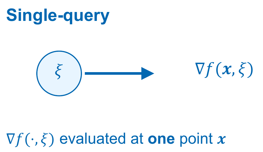
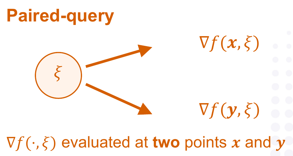
In the single-query protocol, each evaluation uses a fresh sample. The algorithm can keep every previous gradient and use that history to choose the next point. In the paired-query protocol, each fresh sample gives two gradients, typically at the current and previous points. An even more flexible protocol, adaptive reuse, lets the algorithm retain a sample and choose where to query it later, after seeing its earlier answers. In all three cases, we count one query per gradient evaluation, so a pair costs two.
Why might a pair be unavailable? Consider an online production controller that adjusts inventory thresholds. The observed operating window can help estimate how performance depends on the thresholds that were actually used. To pair that observation, we would need to run the same window under different thresholds, from the same starting state and under the same random disturbances. The controller only sees the production line that actually ran. A second evaluation would require a replay mechanism or a model. Even when we can replay the inputs, the second evaluation can require another expensive solve. Yu and Cassandras, §5
Two ways a stochastic gradient can vary
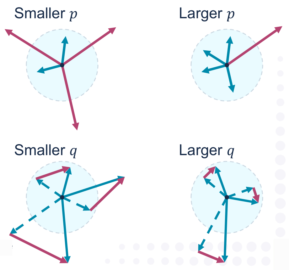
Fix the point and change the sample. The exponent $p$ (with $1<p\le 2$) controls how large the error can get:
\[\left(\mathbb E\lVert g(x,\xi)-\nabla F(x)\rVert^p\right)^{1/p}\le \sigma.\]At the same scale $\sigma$, a larger $p$ gives tighter control of very large errors. Ordinary fluctuations can still be substantial, and for $p<2$ the variance can be infinite.
Fix the sample and change the point. The exponent $q$ controls how much its gradient changes as we move. For finite $q\ge 1$, the condition is
\[\left(\mathbb E\lVert g(x,\xi)-g(y,\xi)\rVert^q\right)^{1/q} \le \bar L\lVert x-y\rVert .\]This is $q$-weak average smoothness. A larger $q$ gives tighter control of unusually large changes. At $q=\infty$, the bound holds almost surely for each fixed pair of points. Additive noise gives a useful example: if $g(x,\xi)=\nabla F(x)+z(\xi)$, the noise can be heavy-tailed, yet it cancels completely in the same-sample difference. Taking the mean in the smoothness bound also gives $\lVert \nabla F(x)-\nabla F(y)\rVert\le \bar L\lVert x-y\rVert$.
Where does a second query help?
Prior work obtained matching paired-query rates with $1\le q\le 2$ under its query model. We obtain the optimal single-query rate and extend the paired rate across the full smoothness range. Two queries per sample also match the best worst-case order under adaptive reuse. Fradin et al.
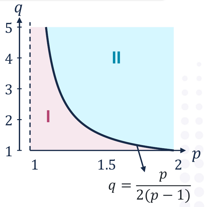
Why does the graph have this shape? Start with what a single-query method can do with its history.
With one query, averaging buys accuracy but costs movement
A standard starting point is normalized SGD with momentum. At iteration $t$ it blends its previous estimate $v_{t-1}$ with the fresh gradient and takes a step of length $h$ in the estimated descent direction:
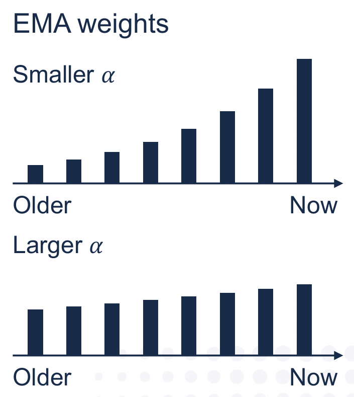
\[\begin{aligned} v_t &= \alpha v_{t-1}+(1-\alpha)g(x_t,\xi_t),\\ x_{t+1} &= x_t-h\frac{v_t}{\lVert v_t\rVert}. \end{aligned}\]The weight on a gradient from $k$ steps ago is $(1-\alpha)\alpha^k$. A larger $\alpha$ gives older observations more influence. Averaging more of them reduces sampling error. But the gradient from $k$ steps ago was estimating the mean at $x_{t-k}$. That mean can be as much as $\bar Lkh$ away from the current mean. To make a long history useful, we may need to move more slowly.
Different parts of a gradient can use different histories
A rare large deviation needs many samples to estimate its contribution to the mean. Can we look further back for that part, while using recent data for the regular part?
We first subtract a rough gradient prediction $w_t$ from the fresh gradient. This gives a residual $u=g(x_t,\xi)-w_t$. We split it with increasing clipping radii $\tau_0,\tau_1,\ldots,\tau_J$. The map $\mathrm{Clip}_\tau$ shortens a vector to length $\tau$ if it is longer, preserving its direction. Define the inner layer $D_0$ and the outer layers $D_j$ for $1\le j\le J$ by
\[\begin{aligned} D_0(u)&=\mathrm{Clip}_{\tau_0}(u),\\ D_j(u)&=\mathrm{Clip}_{\tau_j}(u) -\mathrm{Clip}_{\tau_{j-1}}(u). \end{aligned}\]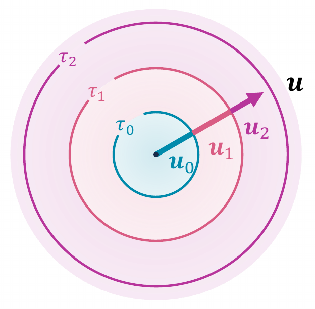
At a given step, we compute every layer from the same batch of fresh gradients. If $z_{j,t}$ is the batch average of layer $j$, we update its estimate as
\[y_{j,t}=\alpha_j y_{j,t-1}+(1-\alpha_j)z_{j,t}.\]We use the current average for the innermost layer and can use longer histories for outer ones. Adding the layer estimates back to $w_t$ gives the direction for a normalized step. The layers add up to the residual clipped at the largest radius. That last cutoff is chosen to keep the contribution left out by clipping small.
There is a reason the outer histories can be longer. Imagine evaluating the same sample at two nearby points, with both predictions fixed, to compare the two layer means. If both residual lengths stay below $\tau_{j-1}$, layer $j$ is zero at both points. Its mean can change only through samples that reach the layer at one point or the other. If that has probability $\pi_j$, Hölder’s inequality gives
\[\left\|\mathbb E[D_j(u')-D_j(u)]\right\| \le \lVert u'-u\rVert_{L^q}\,\pi_j^{\,1-1/q}.\]Here $\lVert u’-u\rVert_{L^q}$ is the same $q$-moment norm as above, applied to the difference of the residuals. The residual moment bound makes $\pi_j$ small for high thresholds, and the increment bound controls how much those residuals can change. The analysis uses this comparison to justify a longer history. The algorithm itself evaluates each sample once. There is no such rarity factor in the regular layer. Many samples can move a little in the same direction, so the regular part of the mean may move even when large changes are tightly controlled.
With a pair, we can correct the old estimate
The picture below takes us back to the first question. The top edge compares two gradients with both the point and the sample changed. A paired query supplies the bottom corner: a gradient at the old point $x_{t-1}$ evaluated with the fresh sample $\xi_t$. On the orange edge only the point changes.
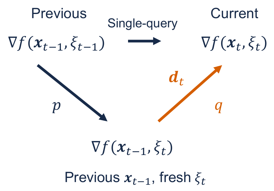
The last equality holds because both points are fixed before the fresh sample is drawn. Think of $v_{t-1}+d_t$ as moving the old estimate forward before blending it with the new reading. The basic update is
\[v_t=\alpha(v_{t-1}+d_t)+(1-\alpha)g(x_t,\xi_t).\]The extra difference is noisy, but its conditional mean is the shift we need. If the old estimate were exact, the updated estimate would be correct on average. The $q$ condition limits the error introduced by the differences. This is the idea behind STORM. Our paired methods use clipping to handle heavy tails. For $q>2$, we apply the correction to each layer, including the regular one, so each layer estimate follows its own moving mean.
Reading the rates
There are two parts to the evaluation cost. Even at one point, we need enough data to estimate a heavy-tailed mean. If $S=\max(1,\sigma/\epsilon)$ compares the noise scale to the target accuracy, that cost is of order $S^r$, where $r=p/(p-1)$. There is also the cost of making progress across many points. Its scale is set by $A=\bar L\Delta/\epsilon^2$, where $\Delta$ bounds the initial objective gap.
| Query protocol | Optimal worst-case number of gradient evaluations |
|---|---|
| Single query | $S^r+AS^{\max(2,r/q)}$ |
| Paired query | $S^r+AS^{\max(1,r/q)}$ |
| Adaptive reuse | $S^r+AS^{\max(1,r/q)}$ |
These are matching upper and lower bounds up to constants depending on $p,q$, for sufficiently large $A$. They count evaluations for expected gradient norm at most $\epsilon$ in the worst case over dimensions. At $q=\infty$, take $r/q=0$.
- Region I, $q\le r/2$. Rare large deviations set the cost of moving through the problem. A single-query method can average these deviations over longer histories, reaching the same order as pairing. The term $AS^{r/q}$ appears in all three rates.
- Region II, $q>r/2$. Regular fluctuations limit single queries. Their cost of progress stops improving at $AS^2$. Paired queries can correct the movement of the mean, so their cost can continue to fall to $AS$ once $q\ge r$. The common $S^r$ cost can still dominate the total.
For example, at $p=q=2$ with fixed positive noise, smoothness and initial gap, the costs grow as $\epsilon^{-4}$ and $\epsilon^{-3}$ for single and paired queries, respectively. The second rate counts both evaluations in every pair. This is the single-versus-paired comparison raised for mean-squared smoothness by Arjevani et al., §6.
Could a clever single-query algorithm avoid the floor altogether? The lower bound hides a sequence of directions the algorithm needs to learn in fresh Gaussian noise. Learning each new direction costs queries even though the noise would cancel in a same-sample difference. A different hard family limits adaptive reuse: returning to a record can expose more of it, but obtaining new independent evidence about a particular hidden block takes a fresh record. These limits are why two evaluations per sample suffice for the optimal order under reuse.
Code, proofs, and paper
The main rate statements are formalized in Lean 4, v0.4.0. The proof guide is plain Markdown for AI assistants and readers who want to trace the assumptions and proof steps to the checked declarations.
Our paper is in preparation. It will give the full mathematical statements, algorithms, and proofs.